A travelogue by Faraz Faheem
Tour du Mont Blanc Day 1: The Union (London -> Geneva -> Chamonix)
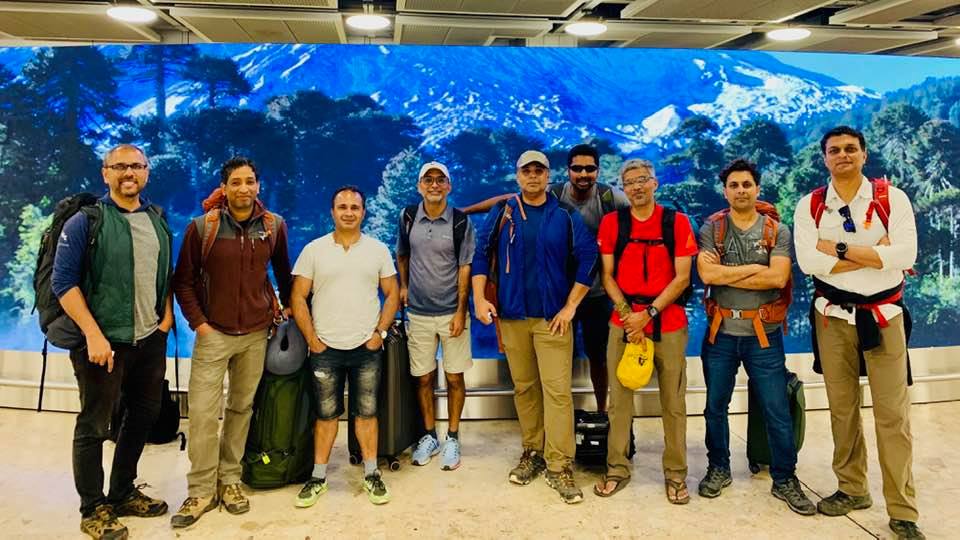
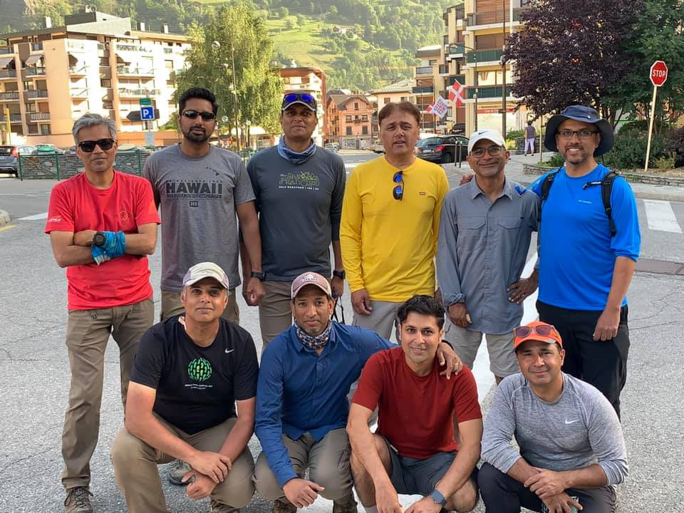
After witnessing Pakistan beat South Africa at Lords Cricket Stadium and a sumptuous buffet at Royal Nawab the previous night, the London group assembles at Heathrow over breakfast. We lost Saqib here due to a family emergency. Samir broke out from his family vacation in Paris and joined us at Geneva Airport. We took a train to the Geneva City Center from where we had to catch the bus to Chamonix. It was one of the hottest day in Geneva and we had a couple of hours to kill. So we decided to take a walk to the Geneva Lakefront and managed to take some group snaps with Geneva Water Fountain in the background. Mo and Laiq went on to grab shawarma wraps for the group. We managed to take a small lunch break under shade in a park next to the bus station before boarding the Flix bus to Chamonix. Umer Mirza travelled from Aarau (close to the Swiss German border) to join us at the hotel. The group was complete.
We had a relaxing evening stroll around this gorgeous mountain town and ended up having a hearty dinner at one of the many Pizzerias at Chamonix City Center. Mo and UK opted for Indian and Turkish meals to satisfy their desi taste buds. It was time to get ready for next morning and catch up on the sleep …
Tour du Mont Blanc Day 2: Shaky Beginning (Chamonix -> Les Houches -> Les Contamines)
Day 2 was an emotional roller coaster. A lot of us jumped into this endurance challenge without much training post Ramadan. Last few days of long distance travels, lack of training and scorching heat was further aggravated by rookie mistakes including delayed start, underestimating the distance and terrain, extended snack and lunch breaks, ignoring the minor planning details etc.
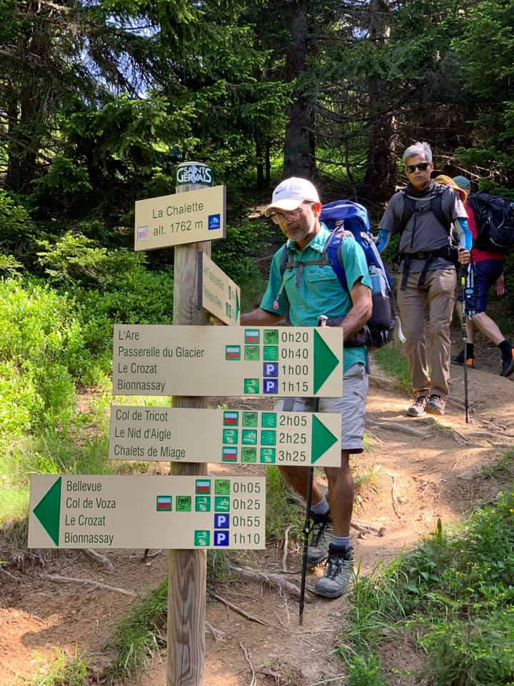
We had a late breakfast, left our surplus luggage at the hotel baggage storage and managed to take the Chamonix Bus to Les Houches after some confusions about the bus stop and bus timing. From Les Houches it was a smooth cable car ride to Bellevue from where the trek began. The first part was a slow and gradual ascent to Cole de Tricot, which would be the highest elevation we gain on this day. The views from Cole de Tricot were amazing and the extreme heat was being perfectly balanced out by the cool glacial breeze. We ended up staying here for about an hour before starting to descend down to the valley below along the Miage glacier. This was a knee wracking and highly technical descent, it was getting late in the afternoon and Mercury was rising above 90s. We all reached down to Refuge de Miage and crashed there. It was a pleasant surprise to find out that they have full service lunch. The cheese and potato omelet, Cup du Miage (berries and cream) and Fromage Blanc felt heavenly after that exhausting descent.
After refilling our water reservoirs we started the second half of the day. We had totally underestimated this part in our planning as it involved 1000+ ft ascent and descent before we reach our destination for the day Les Contamines. Mercury was nearing the 100s, everyone was exhausted, I must say this was the most uneventful and miserable few hours of the entire TMB adventure. The group had started to fall apart emotionally, as the physical and mental endurance limits were challenged, the happy bunch had started to become edgy. That’s where the sound of church bells in the town of Les Contamines served as the glimmer of hope that we are almost done for the day, only to find out later that we are not staying in Les Contamines but at Notre-Dame de La Gorge which is another 1.5mi.
Long story short we checked in Gite Le Pontet, which was our refuge for that night, freshened up, had a decent dinner (the Mung Bean salad was the highlight) and crashed in our dorm beds …

Tour du Mont Blanc Day 3: Getting the Act Together (Notre-Dame de la Gorge -> Les Chapeaux -> Bourg Saint Maurice)
Day 3 was supposed to be the toughest day by the books with nearly 13 miles, 4200 ft of technical climb involving steep glacier trek and 3500 ft descent. We could not afford the rookie mistakes like the previous day today as there was a taxi scheduled to pick us up at 6pm from Les Chapeaux and drop us at our hotel for the night at Bourg Saint Maurice. If we miss the transfer we would be left stranded in the middle of nowhere as Les Chapeaux only had one Refugio which was full. We all assembled the previous night reading up every minor detail for the day and budgeted our time between the segments as well as the stopovers. Mo and Kashif made a wise decision to take a transfer to meet us at Les Chapeaux as they were still sore and cramped up from the previous day and we could not afford to deal with any uncertainties. We had our act together and had to be disciplined throughout the day to execute to the plan.
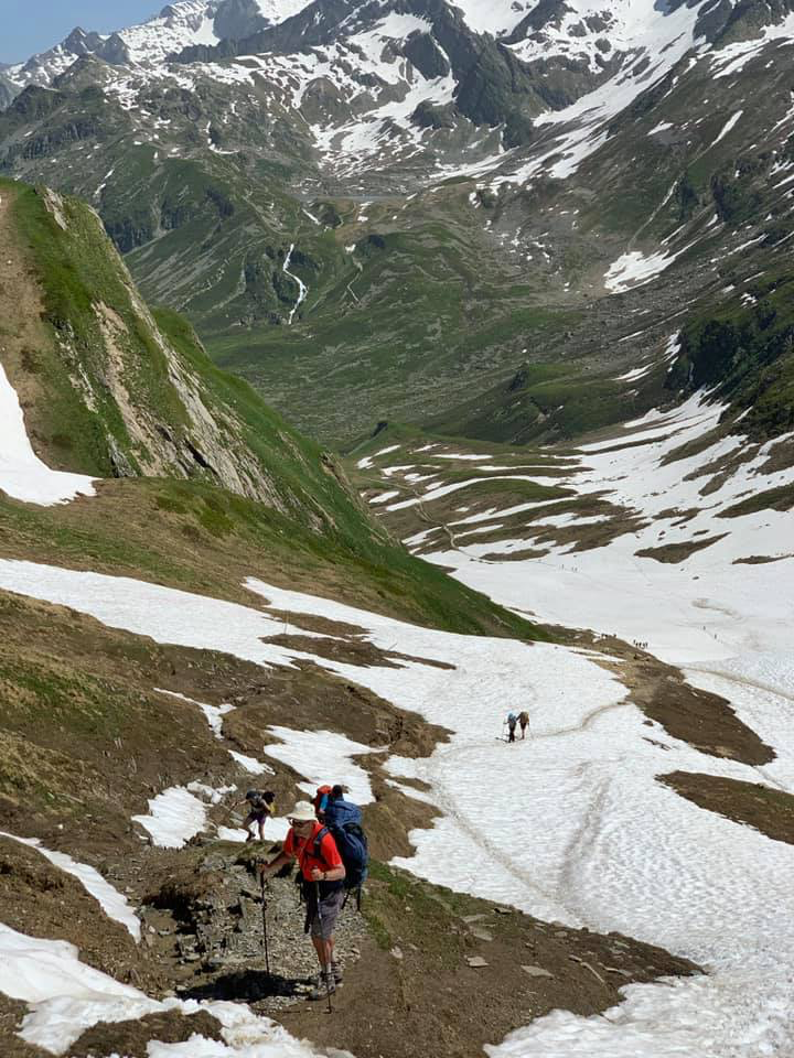
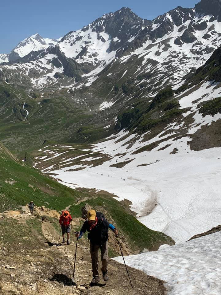
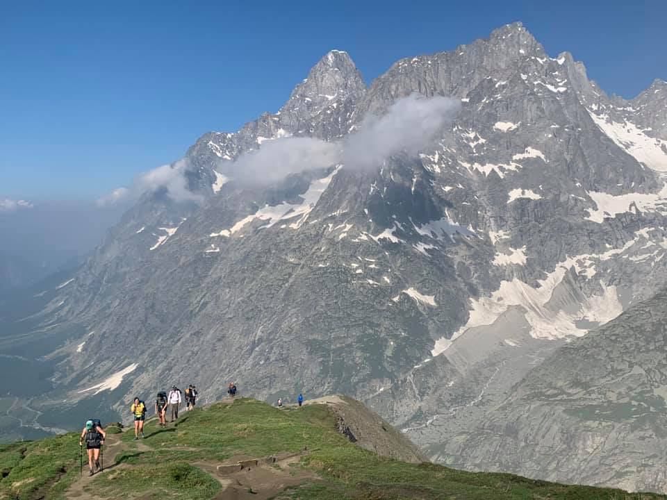
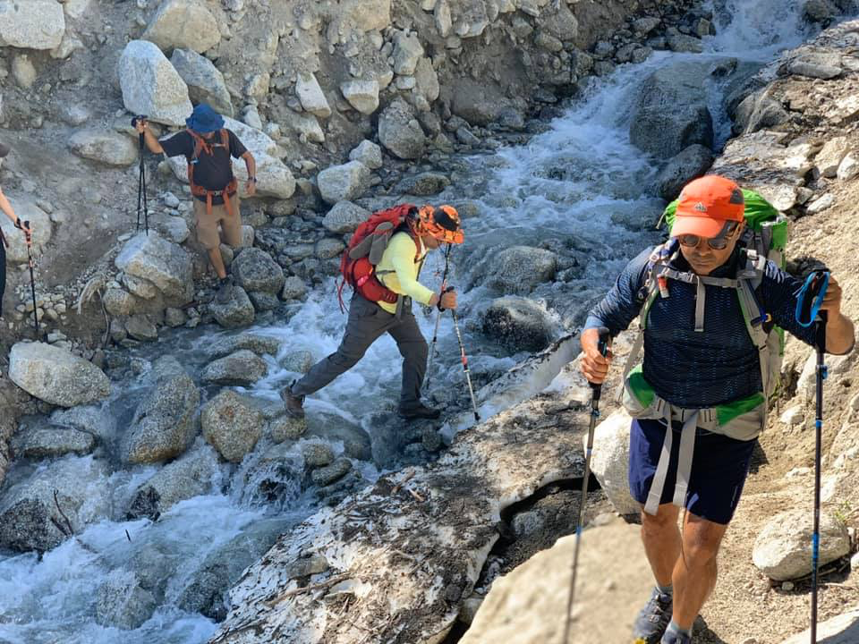
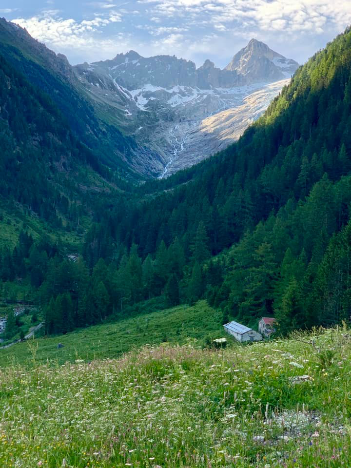
We all woke up early and were ready to start the trek before assembling for breakfast at 7am. First destination of the day was the Church of Norte-Dame de la Gorge. It was a 20 min walk from our dorm. Took a 15 min picture break here and we were off to the mammoth trek. The path gradually ascended along a rushing creek and ended up in a beautiful alpine meadow and grazing fields. The wildflower bloom, sound of cow bells and pleasant breeze all were augmenting the beauty of the scenery. After crossing the footbridge over a small glacier, the path ascended to Refuge la Balme which was our first stop of the day and we were ahead of our time budget. After la Balme the path climbed a bit more and took us to a mound of stones called Tumulus Plan des Dames. The legend is that this is the burial site of an English woman and her servant and all passerby’s put a stone on the tomb to avoid bad luck. A little distance from this point we reached the foot of a glacier beyond which we could see nothing but a steep icy climb to Cole de la Bonhomme. All of us managed to navigate our way up the glacier in a very decent amount of time as the muscles very getting used to the brutal ascents by now. The scenery throughout this segment more than made up for the difficulty of the ascent. We decided to take a small snack break here as the views were breathtaking. Now was the true test as exhaustion was kicking in and the highest point we had to reach was still a couple of miles and some 500-1000ft away. The group did well overall. I hit altitude sickness during this section of the hike and was very very sick by the time we reached the Refuge at Croix du Bonhomme. However we were all happy that we were still tracking the budgeted time very well up to this point. We took a more liberal break here. Here onwards was a 3500 ft descent to Les Chapeaux. As we lost elevation I started to feel a lot better and in an hour or so regained my lost energy. That’s where I looked around the gorgeous green pastures and green mountains all around with the town of Les Chapeaux looking deceptively close even though it was still miles away. It was a very pleasant and gradual descent up until we reached the town. Mo and Kashif joined us hereZ It was still 1.5 hours till our taxi arrives. So we crashed at Auberge la Nova where the taxi was supposed to pick us up from. Some of us decided to visit a small store selling the local yogurt, cheese and jams from the region of Savoie. That’s where a lady checked with me if I am waiting for a taxi as there is a driver who is looking for a party of 11. It was still an hour left till our scheduled pickup time. So it was a bit of surprise. But apparently the driver told me that the pickup time they had with them for our party was 5pm – we lucked out here as if the taxi had left we were kind of stuck in this town without any shelter for the night.
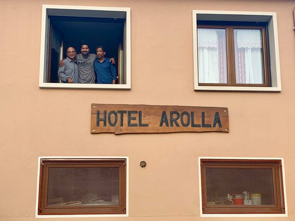
Fast forward an hour we had checked into Hotel Arola at Bourg Saint Maurice. Taqi realized that he had left his shoes back at Les Chapeaux. We asked the taxi driver if it’s possible to go back and pickup the shoes for an extra amount and to our surprise the driver told us that he will be going back to pick up another party in an hour or so and he can bring the shoes back with no extra cost. Our host at Hotel Arola was really helpful with a great sense of humor. He called La Nova Hut and asked them to secure the shoes before the driver arrives to pick them up. It was an amazing experience witnessing how ethical everything is in these mountain towns.
We got together a nearby pizzeria and had pizza for dinner while watching Pakistan beat New Zealand at the ICC worldcup. Then we went on a stroll around the town and picked up ice cream to treat ourselves for a successful day marked by extreme group discipline. We were a team again and ready to embrace and enjoy the 5 days coming ahead …
Tour du Mont Blanc Day 4: Farewell to French Alps (Ville des Glaciers -> La Visaille -> Courmayeur)
This morning Asim and I woke up early morning and decided to take a stroll to the town center to satisfy our caffeine craving. It was our first tutorial for ordering coffee in France. It wasn’t a surprise to find that there was no “Caffe Latte” on the menu which is Italian for “Coffee with Milk”. At the same time we were a bit skeptical about ordering “Caffe au Lait” which is the French for “Coffee with Milk” because in US, Caffe au Lait is literally steamed milk and coffee without any milk foam like latte. But given that we had no other choice we settled for that and to our surprise that was infact what we call Latte in US. Thought it would be a good finding to share for the coffee aficionados traveling from US to France.
By the time we got back to our hotel, we could see the other guys enjoying the views of the town from their hotel room windows. We all got together for breakfast at 7. They had the traditional fare from Savoie region – yogurt, cheese, bread, jam etc. Our host knew we were headed to the mountains in the morning and shared with us the French newspaper with the headline: “even the mountain is not spared by the record heat”. Mother Nature was conspiring against us but we had no option other than to keep marching forward.
8am sharp our taxi came to pick us up and dropped us at Ville des Glaciers, a few km away from the town of Les Chapeaux, where our hike ended the previous night. The first stop was a small scale Beaufort Cheese plant. We did not have the reservation for the tour, but the owner let us freely roam around the production facility and see all the cheese making action live. The effort and passion that guy was putting into cheese making was beyond appreciation and the photographs and video don’t do any justice to that. Not just that but he also let us visit the Cellar where all the goodness was stored for the aging process. Here we got a chance to snap a few group photographs with him. Just look at the smile on his face … kind of an attestation of the fact that small things in life can also make you happy. We wanted to stay longer and learn more about cheese making but it was getting late and heat warning was on. So we decided to packup, got some cheese for the road and hit the trail.
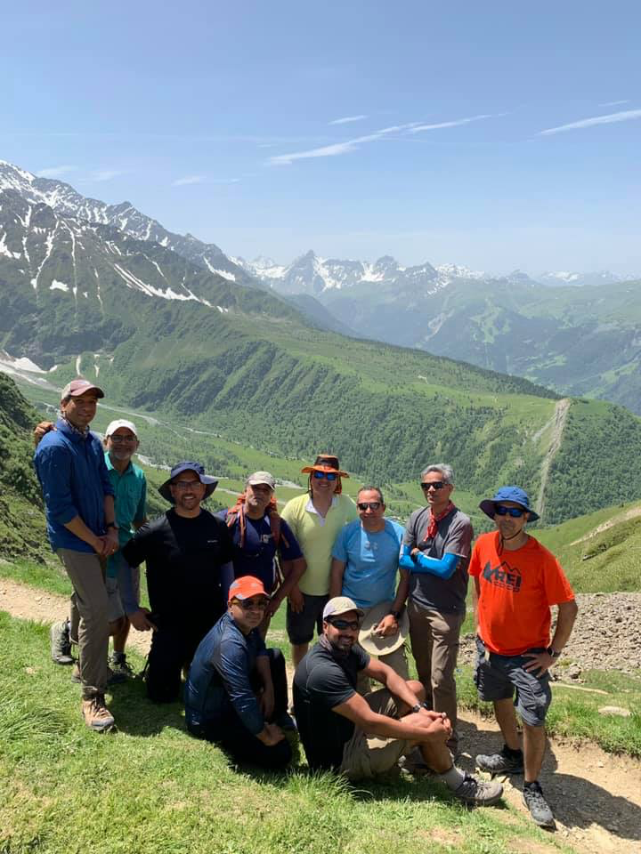
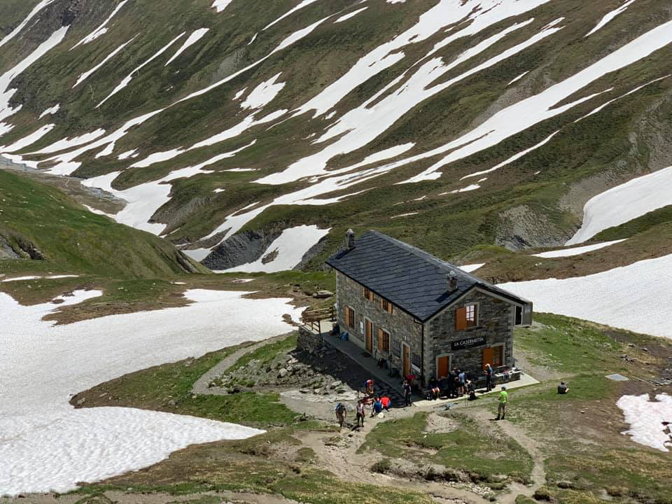
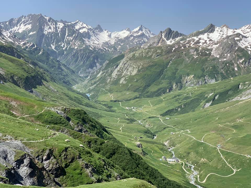
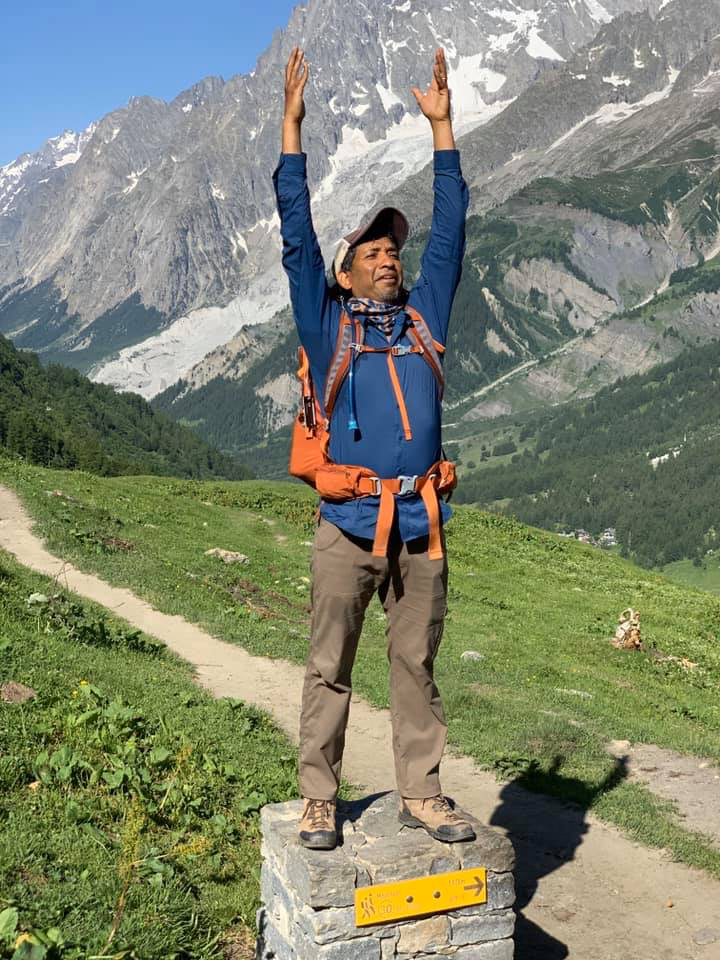
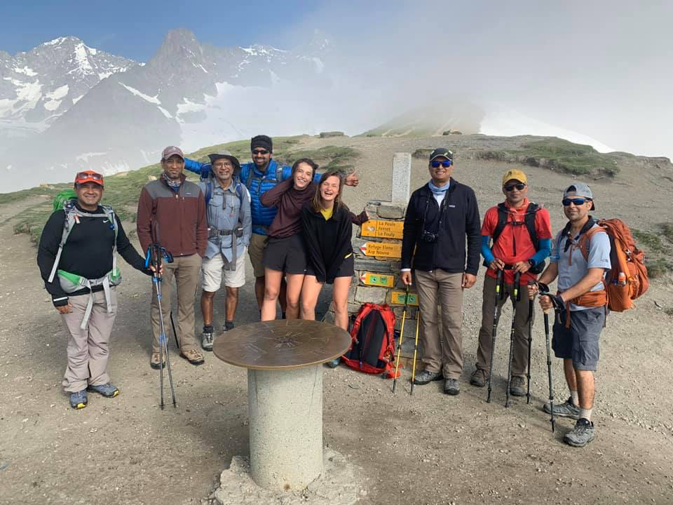
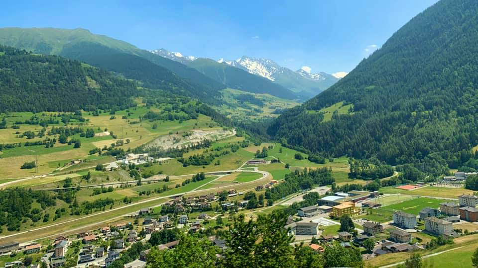
It was a relatively shorter day. First part was a 2 hour ascent to Col de la Seigne at 8200 ft. This was also the border of French and Italian Alps. It was a beautiful ascent with wildflower fields, rushing stream crossings and panoramic valley views. Just before hitting the peak, we stopped at a vista point and took a snack break to absorb the breeze and all the panoramic views. I was expecting large signposts and banners greeting you to Italy but to our surprise if we hadn’t known this is the French-Italian border crossing we wouldn’t even notice we are in Italy now. Took the customary group photographs at Cole de la Seigne and headed down to Refugio Elisasebetta along an icy trek. On the way we saw another mountain hut La Casermetta which turned out to be an environmental education center. There was a model of Mont Blanc and surrounding Alps, also showing the entire route that we were trekking. Also they had a room with pictures and information about all the wildflowers we were witnessing on the way. It was an interesting 15 min break point. After another 45 min or so we reached Refugio Elisabetta, that we could see on top of a mountain towering a few 100 ft above us. As we had already taken some liberal breaks that day, we decided to skip visiting the Refugio and just stayed here long enough for the entire group to reassemble. After this point we had to reach La Visaille from where a short bus ride would bring us to the town of Courmayeur, which would be our stopover for the day. This was a rather uneventful hour long descent to the town of La Visaille all along a paved road and with rising heat and sun shining right on top of our heads, we couldn’t wait to reach our destination for the day.
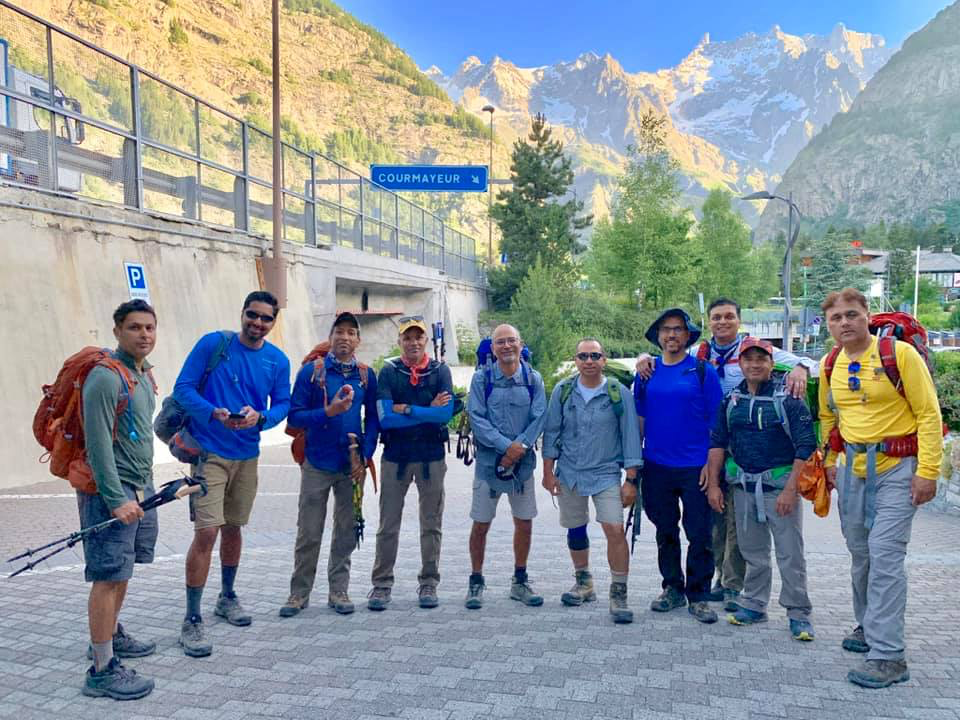
Fast forward we reached La Visaille and took the bus ride to Courmayeur, which is the second major town along TMB after Chamonix and a popular ski resort. After checkin at Hotel Walsser, we had a lot of time to kill until dinner time. The aching body and rising heat outside was telling me to take it easy but the adventurous spirit inside was telling me not to waste any time to explore this beautiful mountain town. So myself and a few of us went for a stroll around the town. The Main Street was a short hike up the hill from the hotel. But I was glad we decided to come here. The pedestrianised street was lined with artisanal shops selling everything from local fare to branded clothing, fancy hotels, cafes and fine dining restaurants. On any day this hands down beats all other skii resort villages I have visited at Tahoe, Whistler and Rockies. We took a relaxing beverage break here before heading back to our hotel.
This was our first dining experience in Italy and the expectations were not that high as we did not opt for the fancier accommodations and meals as part of our tour package. However it turned out to be one of the best sit down dinners we had during the trek. It was a 4 course meal starting with a cheese, salad and fruit buffet followed by soup or pasta, main course and dessert selection. After the food craving was satisfied, we all sat down in the garden outside. The niece of the hotel owner also joined us and shared with us some interesting details about Courmayeur. Also there was a “laundry sorting” ceremony the details of which I would leave out for now. Then it was planning time for next day. If we stick to the plan it was supposed to be another gruelling day with 4000+ ft of elevation gain with the first 2000+ ft gain just in 1-1.5 miles. Not everyone was ready to take on that challenge. So the team split up into two groups – GM, UK and FW decided to stick to the default recommendation whereas the rest of the group decided to breakout and take a short bus transfer to the town of Plampincieux and then hike up 1500 ft to La Leche hut and from there join TMB to continue the journey to our next destination. This alternate recommendation wouldn’t be possible without the help of our host who gave us directions to the minutest possible details which would help us with navigation the next day …
Tour du Mont Blanc Day 5: Wildflower galore in Aosta Valley Italy (Courmayeur -> Refugio Bonatti -> Refugio Elena)
Resuming the account of our memorable adventure after a short sabbatical from my photologues …
We started the morning at Hotel Walsser in Courmayeur with a decent breakfast buffet. The previous night we had decided to split up into two groups to avoid the gruelling 2000ft elevation gain to Refugio Bertone and go for a gentler option from Planpinceaux a short shuttle ride from Courmayeur.
Party A led by Umer left for Refugio Bertone while Party B led by Laiq took the shuttle to Planpinceaux. The idea was to meet-up 1/3rd the way to our final destination, close to La Leche hut, where the switchbacks meet the TMB ridge.
We got dropped off at the stream crossing and started our ascent towards the TMB ridge. Right from the beginning we started witnessing wildflower fields that would last the entire day all the way to Refugio Elena. The initial ascent was under shaded tree canopies and as we were getting closer to the ridge, we got above the tree line and all what we could see was wildflower terraces all the way to the top. It was almost like walking up acres and acres of our very own private garden. It was a relief to see the La Leche hut and the TMB ridge junction shortly after that. We knew we were on the right track …
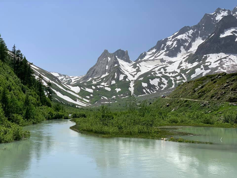
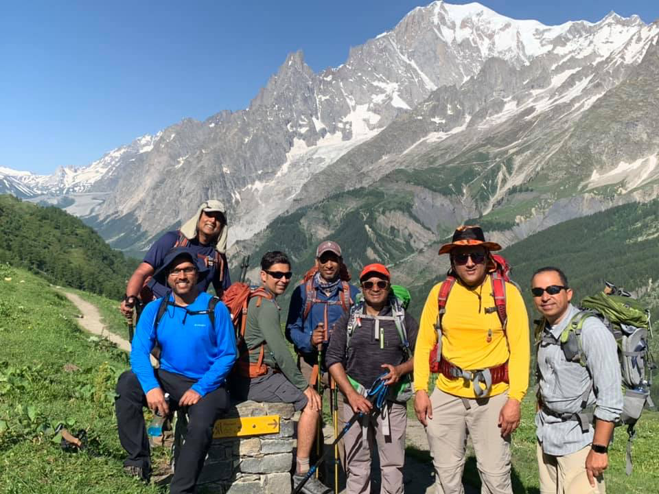
The trail from this point onwards was a wildflower galore as the title and the pictures to follow suggest. The gentle up and down allowed us to enjoy the scenery even more – we were literally walking along an alpine ridge lined up with wildflowers with panoramic views of Vale Ferret to our side with the Southern face of Mont Blanc Massif as the backdrop. A little before noon we reached the foot of a steep hill leading up to the beautiful mountain hut of Refugio Bonatti (as the name suggests). This was our lunch stop for the day and we decided to take an extended break here until the other party joins us.
While we waited for the other party to have lunch together we went for some beverages – the one I found most interesting was a very special Italian soda called “Chinotto” – it’s a bitter-sweet, dark coloured, carbonated drink made of “Chinotto Oranges” with a very distinct taste instead of the typical citrus flavor.
While we were laying down enjoying the views of the Mont Blanc Massif, the other party joined and we went for light lunch – lentil soup and polenta with an assortment of Italian cheeses and bread croutons. After a little more post-lunch siesta we filled up our water reservoirs and resumed our journey down to the valley floor. A noticeable landmark on the way was a footbridge over a gushing waterfall with Himalayan prayer flags tied across. It was a gentle descent down. We reached Chalet Vale Ferret on the valley floor, laid down a bit under the trees and treated ourselves to ice cream before the final and gruelling 1500ft ascent from here to Refugio Elena which was our final destination of the day.
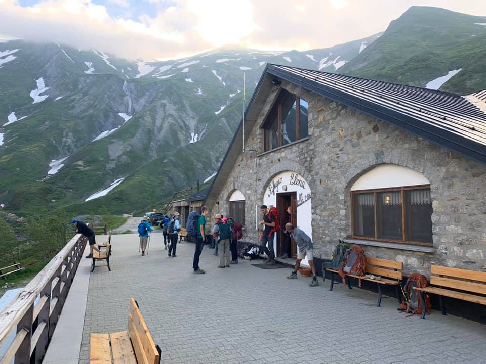
The path leading up to Refugio Elena was a totally exposed, heart pounding grade and the scorching late afternoon sun was not helping make it any easier. But the fatigue was getting perfectly balanced out looking at wildflower terraces all around us, the green and white backdrop of Cole Ferret in front of us and the panoramic views of Vale Ferret on the back. There are couple of difficult glacier crossings on the way specially as the ice was getting slushy and there was a high grade drop on one side. We took a short picture break at a footbridge just before the Refugio and in the next 20 minutes or so we were checking in at the Refugio.
A few of our colleagues had reached there earlier and had checked us all in along with the shower room coins (mostly to regulate the water usage). It was a bunk bed arrangement. We dumped our bags at our spots, took a quick shower break and assembled in the dining room just in time for dinner. It was a much simpler dinner than what we experienced the previous night at Hotel Walsser – still a four course meal with fruits and salad, pasta, entree and dessert. To account for the special dietary needs for our group they had specially prepared chicken just for us.
After dinner we sat together and had a huddle, based on Ghazzali’s suggestion, to reflect on what we have achieved so far, plan for the next day and check on how everyone is doing. Everyone opened up quit a bit about what went wrong and what worked for them and it was a good ice breaker to vent out and settle all the grievances. This was a much needed session as we still had a few more days together and it was the longest everyone had been together on a backpacking trip like this.
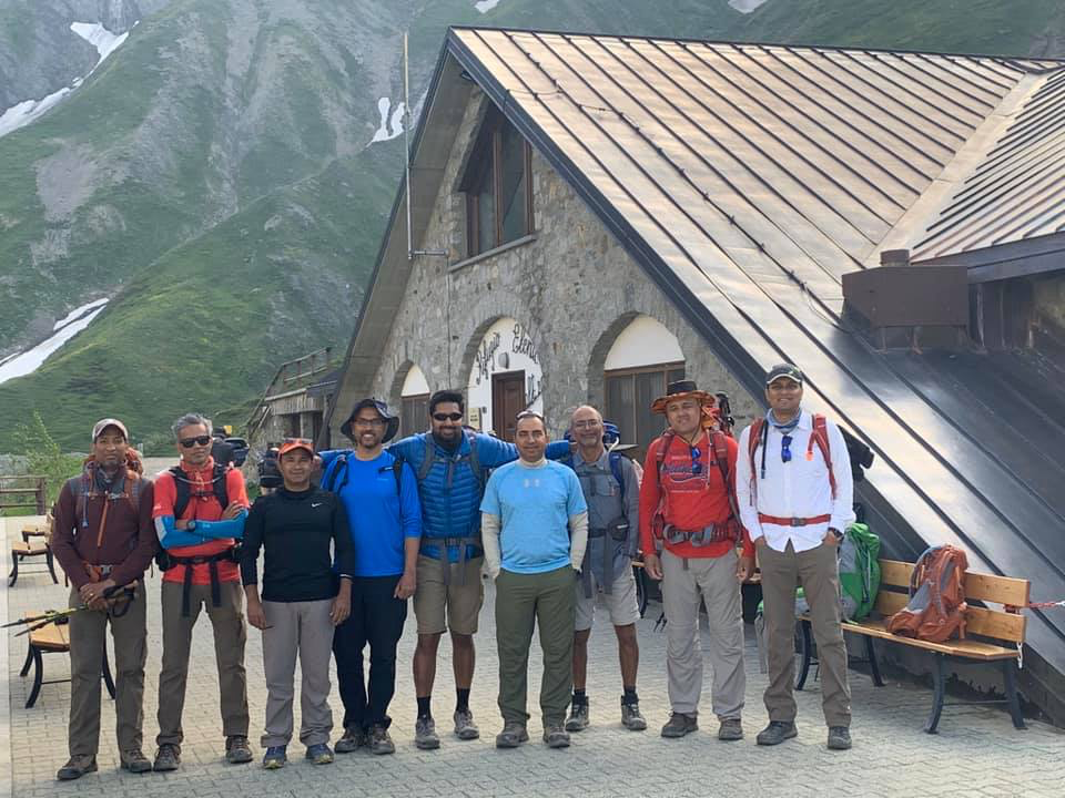
One of the friendly wait staff guy joined us for a group photograph and small talk – “DiDi” if I remember correctly – and invited us to join the smoke session later with the rest of the wait staff outside the Refugio. It was almost like travelling back to my college days hanging out with these college kids who were there to make some extra bucks during Summer to prepare for the Fall semester.
It was getting dark and cold and it was time to call it a night. We crashed in our bunk beds with the sweet dreams about waking up in the cradle of the mountains at 8500 ft. This would be our highest sleepover spot during the trip. Until next day …
Day 6: Switzerland here we come ! (Refugio Elena -> La Peule -> La Fouly -> Champex)
Next morning we woke up early to a misty and foggy morning. We got ready early in the morning and after a quick breakfast, assembled on the patio of Refugio Elena. The low cloud cover was enhancing the majesty of the moment and we could see the path right ahead of us winding up through the mountains to Col Ferret, which was the highest point of our TMB adventure, and also the boundary of Italian and Swiss Alps.
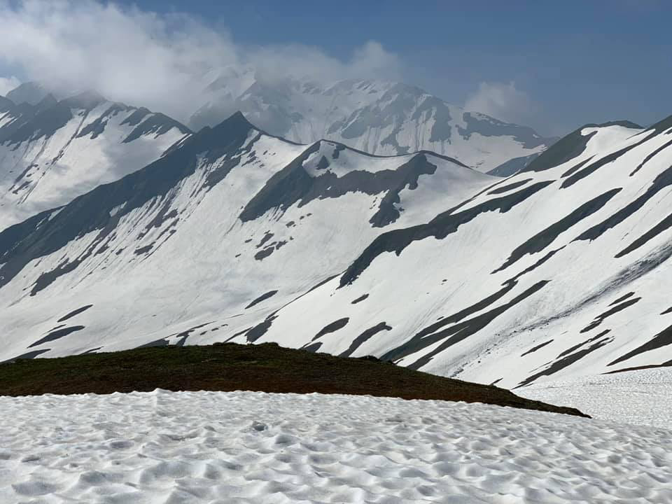
After some steep switchbacks, as the view opened up, all what we could see was the hulking snow covered granite masses of Val Ferret, from the other side of the ridge. We crossed over a steep glacier where the visibility was just a few feet due to the low cloud cover. And then the cloud cover cleared for a few moments for us to witness us standing atop the highest point of TMB – Gran Col Ferret. We spent a few minutes there snapping solos and group pics. A couple of girls from Montana, who we met a couple of times earlier during our TMB circuit as well, joined us for a group pic.
As we started descending from that point we were officially in the Pennine Alps region of Switzerland. Pennine Alps is the western Swiss mountain range bordering Italy with 38 of the 48, 4000m+ peaks in Switzerland (Matterhorn being one of the most noticeable one). The downhill path was all snowy with green and white striped mountains all around us. Even though I was missing the wildflower fields of Aosta valley but this view was uniquely beautiful in its own way, specially, it was a great relief from the heat we had been bearing all along. The icy breeze was pleasantly balancing out the sun, something that can only be experienced and not captured through my iPhone lens.
The first stopover in the Swiss Alps was Refugio La Peule where we stopped briefly for a lunch break to experience some Swiss mountain fare. We got some simple omelet with cheese and tomatoes and the Swiss chocolate milkshake. Again as I described earlier, how the coffee with same name, can have a different meaning in Italy vs France, the same applies to milkshake in Switzerland. It was neither the thick and creamy ice cream shakes that we are used to here in US neither the frappe with the ice slush, instead it was just plain milk shaken with chocolate powder or syrup. It was almost a consistent experience throughout our TMB experience that the focus was few, simple and quality ingredients.
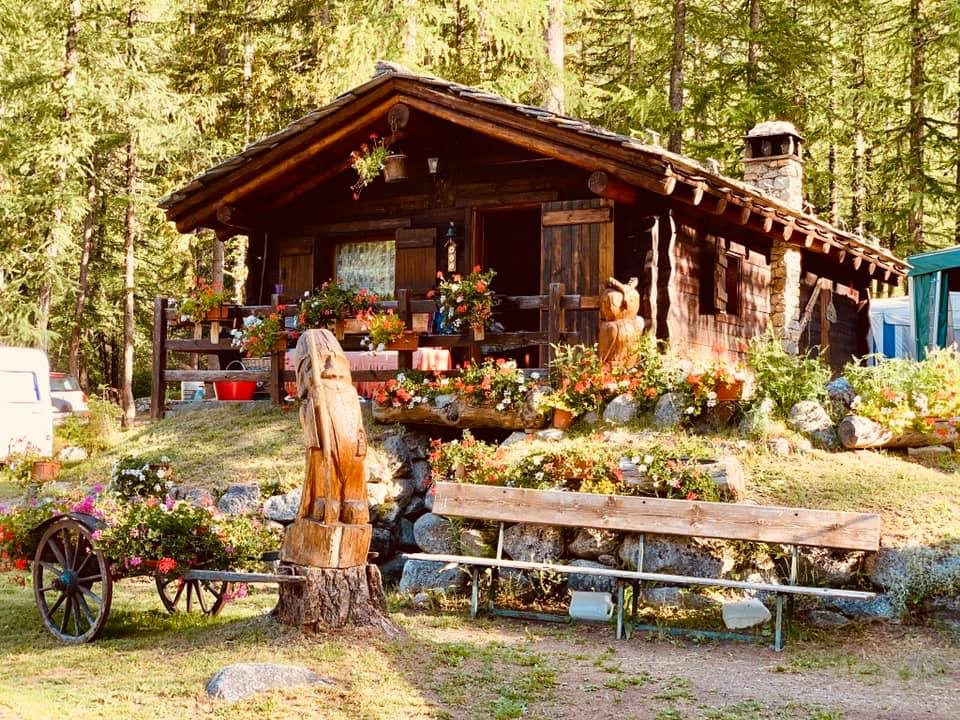
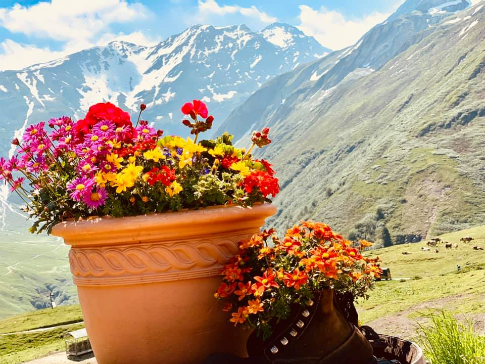
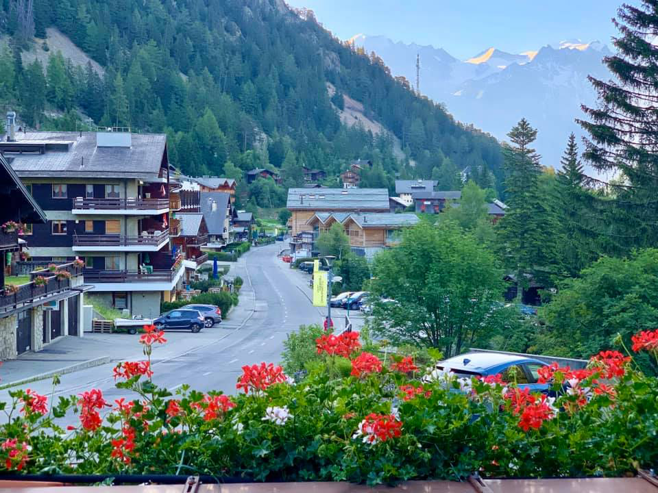
As we descended down from La Peule down to the town of La Fouly we started experiencing a richer Swiss Alps scenery with lush green grazing fields and sounds of cowbells. As we hit the road at the valley floor we saw a couple of very tastefully built cottages with beautifully laid out flower beds and floral pots. Town of La Fouly was still 30 min away. We were supposed to take the bus from La Fouly to Champex but based on the timetable we had already missed the bus and next one was in a few hours. At this point we decided to share a few taxis instead of waiting for the bus. As there was no service, we decided to check for phone service at one of the cottages which seemed like bed and breakfast facility from outside. We saw a maid dressed up in a uniform at the lobby and an elderly gentleman sitting at one of the shaded patios outside having lunch. We ignored the guy and walked straight to the lobby only to figure out later that it was Infact a private home that belonged to the guy we met outside who was an English entrepreneur who chose to retire amidst the Swiss Alps and why not.
In the meantime someone in our group had spotted a taxi outside which was there to pickup another Italian couple who we had met earlier during the trip. Couple of our friends ride shared with them to Champex and the taxi driver asked the rest to meet in the town of La Fouly where he will come and pick us up in another hour. We took the route through the meadows running parallel to the main road and reached La Fouly in no time. The taxi arrived shortly and in next 30 minutes we were dropped off at our hostel in Champex.
After a brief rest, we decided to take a stroll to the lake to cool off and to checkout some water activities. A few of us rented out a stand up paddle board and the rest strolled around the perimeter of the lake. It was a beautiful alpine lake with the back drop of snow capped mountains and colorful buildings with a bunch of lake side cafes and water sport rentals. This seemed like a popular tourist spot along the locals. After a brief walk we decided to settle in at one of the cafes. That’s where Movenpick ice cream sundaes caught our attention. Even though it was getting closer to dinner time at our hostel, it was just too tempting to pass and we decided to go for the ice cream feast.
It was getting late in the evening and cafes and shops around the town had started to close. We headed back to the hostel and gathered at the outdoor patio for some chit chat before dinner was served. It was a relatively simpler meal – chicken and peas risotto followed by a small serving of a triple chocolate mousse. But filling enough, specially after the big servings of ice cream sundaes we had earlier in the evening. We got back to our rooms and crashed on the bed with sweet dreams about what More Switzerland had to offer the next day …
Day 7: A whimsical sleepover in the cradle of Swiss Alps (Champex -> Alp Bovine -> Trient -> La Peuty)
Next day we followed the morning ritual – woke up early in the morning, got dressed up, grabbed quick breakfast and assembled outside the hostel for the mandatory group photograph before we start marching ahead. A few of us got reprimanded by the strict warden about not treating the hostel as our own home eventhough all of us were seasoned hikers and very well aware of the code of conduct at the mountain dormitories and hostels. Just an observation that the overall hospitality experience in Switzerland had not been even close to what we experienced in France and Italy. But again I would give it a benefit of doubt given our sample size was too small to pass a blanket statement.
Anyways shrugging off that small unpleasant incident, we started walking towards the TMB segment leading up to the town of Trient which was our destination for the day. First mile or so was a flat walk across the meadows and then the path started ascending up first gently followed by some steep switchbacks and some wide stream crossings and eventually a long calve-burning ascent up to the Alp Bovine.
We decided to take a lunch break here at Alp Bovine. Other than the usual mushroom and cheese omelet we also ordered Rosti, which was a cheesier and less fried version of what we call hash browns here in US. After lunch we walked over to the other side of the mountain where the panoramic views of Rhône Valley (Martigny) opened up. From a distance we could see the snow capped peaks of the Bernese Alps (Monch, Eiger and Jungrau being the prominent ones).
From here we started to descend towards Col de la Forclaz mountain pass, which connects Martigny to the other French cities all the way to Chamonix, where we started our journey. At Forclaz we had to wait a bit for some of our colleagues who were having knee issues during these steep descents. I grabbed some fresh strawberries, apricot and cherries from a roadside fruit stand that made a perfect mid afternoon snack in this hot weather.
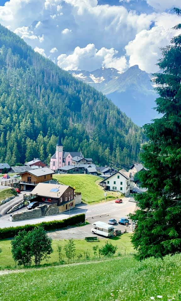
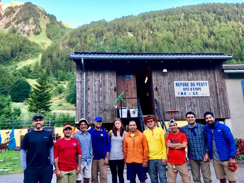
From Forclaz it was another steep descent until we started seeing the panorama of the city of Trient with it’s prominent pink church visible from a distance. In another hour or so we reached the town of Trient. Our final destination of the day was the hamlet of La Peuty which was another mile or so flat walk from Trient. We waited for rest of our colleagues and then started heading towards our final destination of the day.
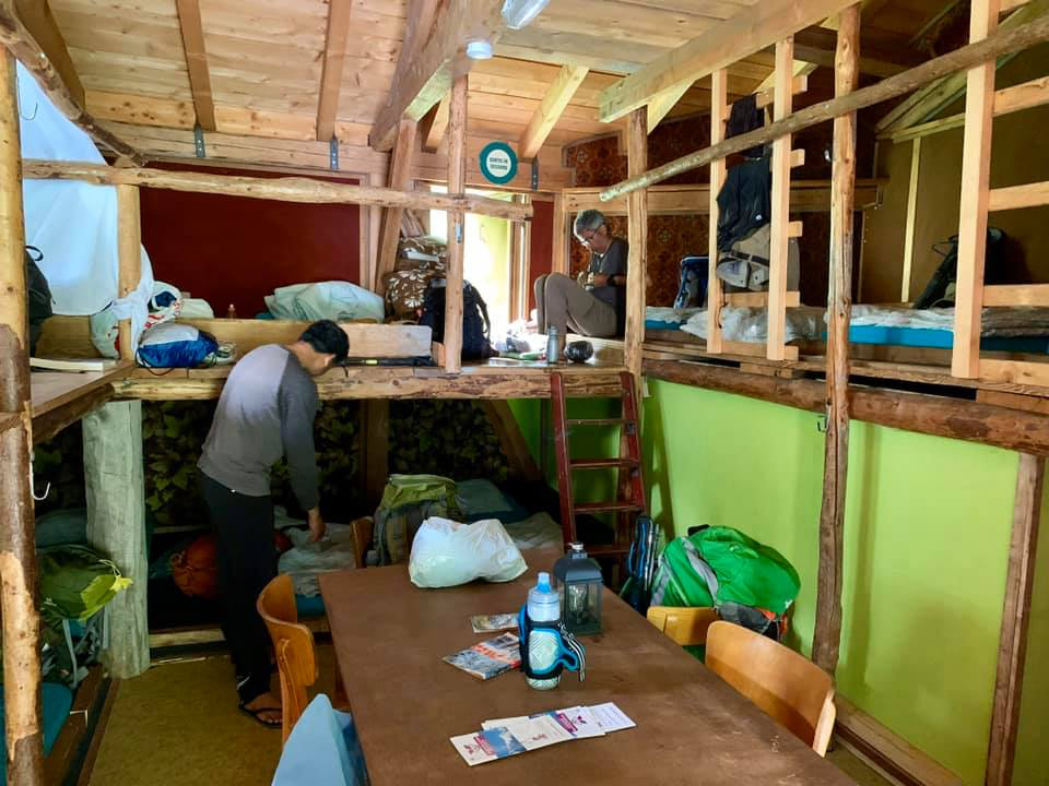
The dormitory style housing at La Peuty was interesting to say the least. It was one large attic with a whole bunch of sleeping mattresses laid out next to each other across two levels. There was a large assembly table in the middle, a place to hang our backpacks and a charging station. The Rifugio was being run by a young Swiss couple – Anja and Rafael. We were greeted there by Anja and her friendly assistant. After checking in I grabbed an iced tea and went to the garden outside for lounging while dipping my feet in the foot bath for some muscle relief. The dormitory was very playfully laid out with a bunch of fun things and activities – including the recliners, the visitor stone pot, the bee house, etc.
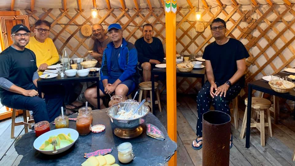
The most noticeable thing was the yurts – one of them was our dining room and another one was a living room with board games and library. Just watch the video as part of the collection to witness the inside arrangements of the yurts.
Dinner was exceptional – starter salad, Thai rice and yellow curry for main course and berry pie for dessert. It was unbelievable to see how the two hostesses were taking care of everything from reception duties to handling the bar to cooking the food and then feeding a whole bunch of hungry hikers without any extended waits to replenish the servings.
After the dinner we decided to take a stroll back to Trient to checkout the town and the church. On the way we saw a field of Lupines in full bloom. We took a few moments to capture the Lupines with a backdrop of snow capped mountains and grassy fields. The church was a beautiful and vibrant pink colored structure and as the sun was setting, it was resulting in a strange glow to the pink color that was accentuating the beauty of a perfect backdrop of a typical Swiss town. There was a graveyard next to the church with some marble and stone graves and tombs which was adding a mysterious vibe to the whole scene.
It was getting dark and we had already heard a few thunders. So we headed back to our dorms. I wasn’t feeling sleepy. So I sat in the garden for a bit just trying not to think about anything and be in the moment. Cloud cover was gathering fast and breeze was picking up. So I decided to go back to my bed. Everyone around me was asleep. The attic windows were open and we could hear the thunder and wind picking up outside. As soon as I laid down the rain started thumping hard on the roof above us. Hard to describe this whole experience. That night I slept like a baby in the cradle of the whimsical Swiss Alps with a melancholic feeling that all this is about to end soon as we start our final leg of the journey the next day …
Day 8: The Finale! (La Peuty -> Col de Balme -> La Tour -> Chamonix)
It’s been the longest most of us had been on the road straight with just our backpacks. Some were getting fatigued, some just wanted to take it easy and avoid another grueling day of hiking, some were feeling homesick and wanted to join their families for the rest of European adventure. Previous night almost half of the group decided to split up and head directly to Chamonix via public transportation and skip the hike.
Next morning when we assembled at breakfast at the yurt, almost everyone had given it a second thought overnight and all except one, decided in favor of finishing strong by embracing the final hike of the day. We were all ready for the “Finale” !
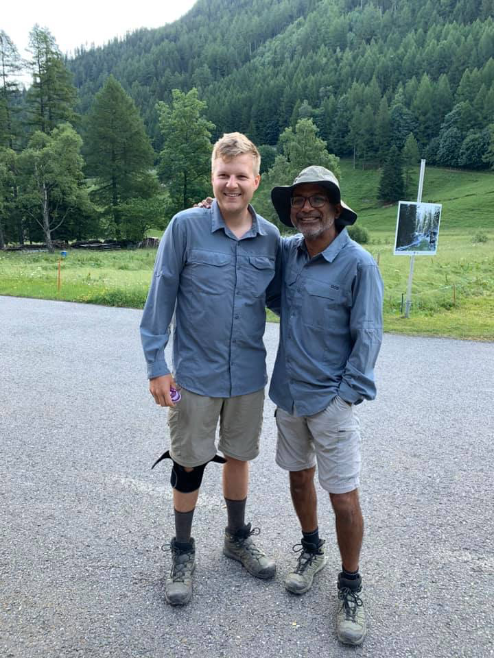
Previous night over dinner we had befriended a family from Minnesota – husband, wife, 3 daughters and son-in-law. They were sharing the dorm room with us. Figured out they had similar plans for the day. Checkout the pic of the son-in-law with Ghazzali – how coincidentally they ended up dressing almost exactly the same way for the day !
The initial path was a very gradual incline through meadows and wildflower flower fields. And then the slope became a lot steeper as we ascended towards Col de Balme which was the final mountain pass on the way before we started heading down to Chamonix valley, where we had started the journey 7 days back.
The mountain hut at Col de Balme was gorgeous and was enhancing the scenery all around us. As we crossed the hut the panoramic views of Chamonix Valley opened up in front of us. We decided to take one final long break here before we say goodbye to TMB. Asim made tea for all of us which just hit the spot.
While we were resting there, the Italian couple with whom we shared the taxi ride to Champex, the family from Minnesota whom we stayed with at La Peuty and all of our group members also joined. We decided to take a group photograph of this one big happy family away from home. Everyone had a big smile on their face – was it sense of accomplishment, anticipation to reach the final destination, to get reunited with the families waiting for us down there in the valley or just the euphoria of the moment l, it’s hard to tell. I wanted to capture the moment forever in my memory, breath all that fresh alpine air, smell all that wildflower aroma around us, continue listening to the silence of the mountains, stare at that beautiful panorama of Chamonix Valley for hours, lay down forever and feel the misty grass. But such is the tyranny of time that such moments don’t last forever and it was time for us to leave. Some of the verses from a Robert Frost poem that I had read a while back echoed in my mind:
“The woods are lovely, dark and deep;
But I have promised to keep;
And miles to go before I sleep;
And miles to go before I sleep”
That moment was so perfect that there was little point left in carrying on the rest of the hike. And most of us, including me, decided to take the cable car down. Took us less than 30 min to reach Chamonix valley. We were at the border town of La Tour and there was a bus to Chamonix waiting for us there. When we reached the town of Chamonix we saw the same signs we saw when we arrived here 7 days back – 10 gelato scoops for 10 Euro. There was no reason to resist that.
We checked in at our hotel rooms and between 12 and 2 all the group members started arriving one after the other. All of us had different plans for the evening. My family had joined me from Geneva. It was time to say goodbye to friends. We hugged and headed down our own ways only thinking about when are we going to do something like this again and if we had achieved nirvana and nothing that we ever do would beat this experience. Well I have yet to figure that out. Until that time Goodbye and enjoy the pics !
For more photos:
https://www.facebook.com/faraz.faheem.9/media_set?set=a.10217158726511737&type=3